ダブルミニマムポテンシャルの数値解
home > 計算物理学 >[サイトマップ]
目次
ダブルミニマムポテンシャル
つぎの式で表されるポテンシャル
は相転移などを議論するとき用いられるもので,ダブルミニマムポテンシャル(二重極小ポテンシャル) もしくはダブルウェルポテンシャル(二重井戸ポテンシャル)と呼ばれるものです.プログラムのポテンシャルの形を書き換え, いくつかの a に対する固有値を求めてみました. 縦軸のスケールは各グラフによって適当に変更しています.
コーディング
アルゴリズム
微分方程式(シュレディンガー方程式)を解くのには 4 次のルンゲ・クッタ法を使います.
ソースコード
     1  /* =====================================================================
     2     Runge-Kutta法でダブルミニマムポテンシャルの固有値を求める
     3     Last modified: May 28 2003
     4     ===================================================================== */
     5
     6
     7  #include <stdio.h>
     8  #include <math.h>
     9  #include "cpgplot.h"
    10
    11
    12  // 物理設定
    13  double E = 0;
    14  double dE = -1.0;
    15  int parity = 1;
    16
    17  // きざみ幅
    18  double h = 0.001;
    19
    20
    21
    22	/* ---------------------------------------------------------------------
    23	   potential function
    24	   --------------------------------------------------------------------- */
    25
    26	double V(double x){
    27	  // V(x) = x^4 - ax^2
    28	  return (pow(x,4) - 0*pow(x,2));
    29	}
    30
    31
    32
    33	/* ---------------------------------------------------------------------
    34	   導関数の定義
    35	   --------------------------------------------------------------------- */
    36
    37	double dphi(double x, double phi, double z){
    38	  // dphi/dx = z
    39	  return(z);
    40	}
    41
    42	double dz(double x, double phi, double z){
    43	  // dz/dx = (V(x)-E)phi
    44	  return((V(x) - E) * phi);
    45	}
    46
    47
    48
    49	/* ---------------------------------------------------------------------
    50	   Runge-Kutta法
    51	   ---------------------------------------------------------------------- */
    52
    53	void rungeKuttaMethod(double x0, double phi0, double z0, double h){
    54	  int i, j, n, loop, color;
    55	  double x, phi, z, k[4], q[4], phi_old[2];
    56	  loop = 15/h; color = 9;
    57
    58	  for(n=1 ; n<=14 ; n++){
    59	    dE = -1 * dE/10;
    60	    x = x0; phi = phi0, z = z0;  // 波動関数初期化
    61
    62	    while(1){
    63	      for(i=1 ; i<=loop ; i++){
    64		// 4次のRunge-kutta法 の連立
    65		k[0] = h * dphi(x, phi, z);
    66		q[0] = h * dz(x, phi, z);
    67		k[1] = h * dphi(x + h/2, phi + k[0]/2, z + q[0]/2);
    68		q[1] = h * dz(x + h/2, phi + k[0]/2, z + q[0]/2);
    69		k[2] = h * dphi(x + h/2, phi + k[1]/2, z + q[1]/2);
    70		q[2] = h * dz(x + h/2, phi + k[1]/2, z + q[1]/2);
    71		k[3] = h * dphi(x + h, phi + k[2], z + q[2]);
    72		q[3] = h * dz(x + h, phi + k[2], z + q[2]);
    73		phi += k[0]/6 + k[1]/3 + k[2]/3 + k[3]/6;
    74		z   += q[0]/6 + q[1]/3 + q[2]/3 + q[3]/6;
    75		x = x0 + i * h;
    76	      }
    77	      // 今回と前回のphiを保存
    78	      phi_old[0] = phi_old[1]; phi_old[1] = phi;
    79
    80	      // 今回と前回のphiが異符号ならwhile(1)を抜ける
    81	      // i=1ではphi_oldの値が無意味なので比較しない
    82	      if ( (i>=2) && ((phi_old[0] > 0) && (phi < 0)) ) break;
    83	      if ( (i>=2) && ((phi_old[0] < 0) && (phi > 0)) ) break;
    84
    85	      printf("%2.15lf\n", E);  // モニタ
    86	      E += dE;  // 固有値変更
    87	      x = x0; phi = phi0, z = z0;
    88	    }
    89	  }
    90
    91	  // 波動関数の描画
    92	  x = x0; phi = phi0, z = z0;
    93	  for(i=1 ; i<=loop ; i++){
    94	    k[0] = h * dphi(x, phi, z);
    95	    q[0] = h * dz(x, phi, z);
    96	    k[1] = h * dphi(x + h/2, phi + k[0]/2, z + q[0]/2);
    97	    q[1] = h * dz(x + h/2, phi + k[0]/2, z + q[0]/2);
    98	    k[2] = h * dphi(x + h/2, phi + k[1]/2, z + q[1]/2);
    99	    q[2] = h * dz(x + h/2, phi + k[1]/2, z + q[1]/2);
   100	    k[3] = h * dphi(x + h, phi + k[2], z + q[2]);
   101	    q[3] = h * dz(x + h, phi + k[2], z + q[2]);
   102	    cpgsci(color); cpgmove(x, phi); cpgdraw(x + h/6, phi + k[0]/6);
   103	    cpgsci(color); cpgmove(x + h/6, phi + k[0]/6); cpgdraw(x + h/2, phi + k[1]/2);
   104	    cpgsci(color); cpgmove(x + h/2, phi + k[1]/2); cpgdraw(x + h*5/6, phi + k[2]*5/6);
   105	    cpgsci(color); cpgmove(x + h*5/6, phi + k[2]*5/6);  cpgdraw(x + h, phi + k[3]);
   106	    phi += k[0]/6 + k[1]/3 + k[2]/3 + k[3]/6;
   107	    z   += q[0]/6 + q[1]/3 + q[2]/3 + q[3]/6;
   108	    x = x0 + i * h;
   109	  }
   110
   111	  // 求まった固有値を表示
   112	  printf("E = %2.15lf\n", E);
   113	}
   114
   115
   116
   117	/* ---------------------------------------------------------------------
   118	   ポテンシャルの形を描画
   119	   --------------------------------------------------------------------- */
   120
   121	void drawPotential(double xmax)
   122	{
   123	  double i;
   124	  cpgsci(4); cpgslw(1);
   125	  cpgmove(-xmax, pow(xmax,2)/2);
   126	  for(i = -xmax ; i < xmax ; i += 0.1){
   127	    cpgdraw(i, pow(i,4) - 0*pow(i,2));
   128	  }
   129	}
   130
   131
   132
   133	/* ---------------------------------------------------------------------
   134	   main
   135	   --------------------------------------------------------------------- */
   136	int main(void)
   137	{
   138	  double phi0, z0;
   139	  double xmax, bottom, top;
   140
   141	  // グラフ描画設定
   142	  xmax   = 4.0;
   143	  bottom = 1.3;
   144	  top    = 1.3;
   145	  cpgopen( "/xserv" );
   146	  cpgpap( 7.0, .6 );
   147	  cpgenv( 0, xmax, -bottom, top, 0, 0 );
   148
   149	  if (parity == -1) {
   150	    phi0 = 0.0; z0 = 1.0;  // 奇関数
   151	  }
   152	  else {
   153	    phi0 = 1.0; z0 = 0.0;  // 偶関数
   154	  }
   155
   156	  drawPotential(xmax);
   157	  rungeKuttaMethod(0., phi0, z0, h);
   158
   159	  cpgclos();
   160	  return 0;
   161	}
実行結果
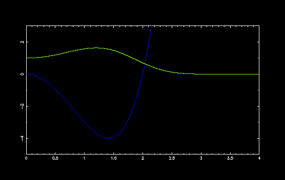
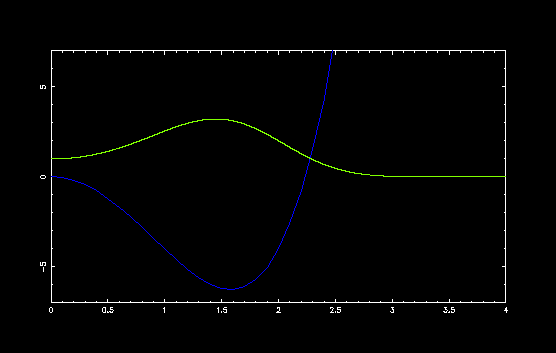
ダブルミニマムポテンシャル V(x) = x4 - a x2 の a の値を変えて,いくつかのポテンシャルで計算してみました.
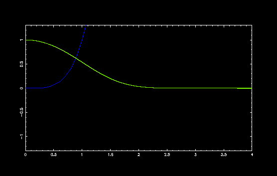
a = 0, E = 1.060362090484170
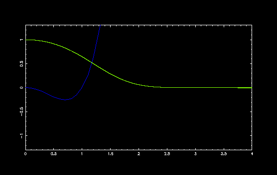
a = 1, E = 0.657653005180699
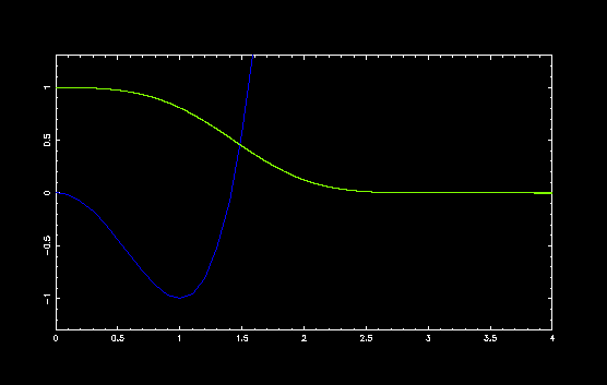
a = 2, E = 0.137785848188210
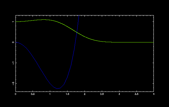
a = 3, E = -0.593493304218450
a = 4, E = -1.710350450132565
a = 5, E = -3.410142761239649
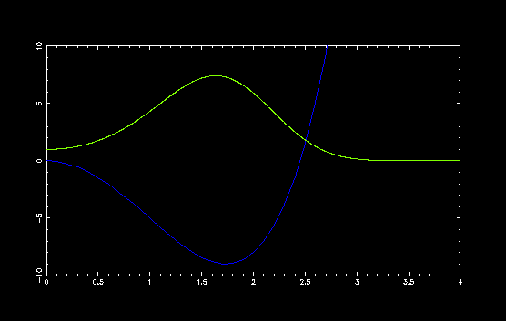
a = 6, E = -5.748190520666807
x = 0 でポテンシャルの山が高くなるにしたがって, 固有値と固有関数が変化する様子がわかります. 中央のポテンシャルの山が高いと古典的には粒子は一方の谷の中央で振動しますから, 量子力学的にも山が高い場合には,それぞれの谷で振動している2つの振動子を考えることができます.